Problem: Your Embeddings Are a Black Box

You've got a vector database full of embeddings — but you have no idea what's actually in there. Are similar documents clustering together? Are there outliers dragging down retrieval quality? You can't answer any of this by staring at 1536-dimensional floats.

UMAP (Uniform Manifold Approximation and Projection) collapses those dimensions down to 2D or 3D while preserving local structure — so you can actually see what's going on.

You'll learn:

How to install and configure UMAP for Python
How to project any embedding matrix to 2D
How to build an interactive plot with color-coded labels
What to look for once you can see your vector space

Time: 20 min | Level: Intermediate

Why This Happens

High-dimensional vectors (256, 768, 1536 dims) are impossible to inspect directly. Most debugging workflows rely on cosine similarity queries — but those only tell you about individual pairs, not the global structure of your data.

UMAP solves this by learning a low-dimensional representation that keeps nearby points close and distant points far. Unlike PCA, it handles non-linear structure well. Unlike t-SNE, it's fast enough to run on 100k+ vectors in under a minute.

Common use cases:

Auditing an embedding model before deploying to production
Finding mislabeled or near-duplicate documents in your corpus
Comparing two embedding models side-by-side
Debugging why retrieval is returning unexpected results

Solution

Step 1: Install Dependencies

pip install umap-learn matplotlib pandas numpy
# For interactive plots (recommended)
pip install plotly

Note: The package is umap-learn, not umap. Installing umap by mistake is one of the most common errors here.

Expected: No errors. If you hit a numba conflict, pin it:

pip install "numba>=0.56,<0.60" umap-learn

Step 2: Load Your Embeddings

UMAP expects a 2D NumPy array with shape (n_samples, n_dimensions).

import numpy as np
import pandas as pd

# Option A: Load from .npy file
embeddings = np.load("embeddings.npy")  # shape: (n, dims)

# Option B: Load from a DataFrame (e.g., from a vector DB export)
df = pd.read_parquet("vectors.parquet")
embeddings = np.stack(df["embedding"].values)

# Option C: Generate on the fly with sentence-transformers
from sentence_transformers import SentenceTransformer

model = SentenceTransformer("all-MiniLM-L6-v2")
texts = ["your", "documents", "here"]
embeddings = model.encode(texts, show_progress_bar=True)

print(f"Embedding matrix: {embeddings.shape}")  # e.g., (5000, 384)

Expected: A NumPy array printed as (n_samples, n_dims).

If it fails:

ValueError: setting an array element with a sequence — your embeddings aren't all the same length. Filter them first.
Memory error on large datasets — sample down to 50k rows for exploration: embeddings = embeddings[:50000]

Step 3: Run UMAP

import umap

reducer = umap.UMAP(
    n_neighbors=15,    # Controls local vs global structure (5-50)
    min_dist=0.1,      # How tightly points cluster (0.0-1.0)
    n_components=2,    # Output dimensions (2 for plotting)
    metric="cosine",   # Use cosine for text embeddings, euclidean for images
    random_state=42    # For reproducible layouts
)

projected = reducer.fit_transform(embeddings)
print(f"Projected shape: {projected.shape}")  # (n_samples, 2)

Parameter guide:

n_neighbors=15 — good default. Lower = tighter local clusters. Higher = more global structure visible.
min_dist=0.1 — lower values pack clusters tighter. Use 0.0 to see maximum separation.
metric="cosine" — use this for text/NLP embeddings. For image embeddings, euclidean is usually better.

Expected: Runs in 10-60 seconds depending on dataset size. You'll see a progress bar from numba.

Step 4: Plot the Results

Static plot (matplotlib):

import matplotlib.pyplot as plt

fig, ax = plt.subplots(figsize=(12, 8))
scatter = ax.scatter(
    projected[:, 0],
    projected[:, 1],
    c=labels,          # Color by category — see below for label setup
    cmap="tab20",
    alpha=0.6,
    s=5                # Point size — reduce for large datasets
)
ax.set_title("Vector Space (UMAP 2D Projection)")
plt.colorbar(scatter, ax=ax, label="Category")
plt.tight_layout()
plt.savefig("vector_space.png", dpi=150)
plt.show()

Interactive plot (plotly — recommended):

import plotly.express as px

plot_df = pd.DataFrame({
    "x": projected[:, 0],
    "y": projected[:, 1],
    "label": labels,       # String categories work here
    "text": texts,         # Hover tooltip
})

fig = px.scatter(
    plot_df,
    x="x", y="y",
    color="label",
    hover_data=["text"],   # Shows the actual document on hover
    title="Vector Space (UMAP 2D Projection)",
    opacity=0.6,
)
fig.update_traces(marker=dict(size=4))
fig.write_html("vector_space.html")  # Open in browser for full interactivity
fig.show()

Setting up labels (if you don't have them):

# From a DataFrame column
labels = df["category"].values

# From a list of strings
labels = ["finance", "tech", "health", ...]

# Numeric cluster IDs (e.g., from k-means)
from sklearn.cluster import KMeans
km = KMeans(n_clusters=10, random_state=42).fit(embeddings)
labels = km.labels_

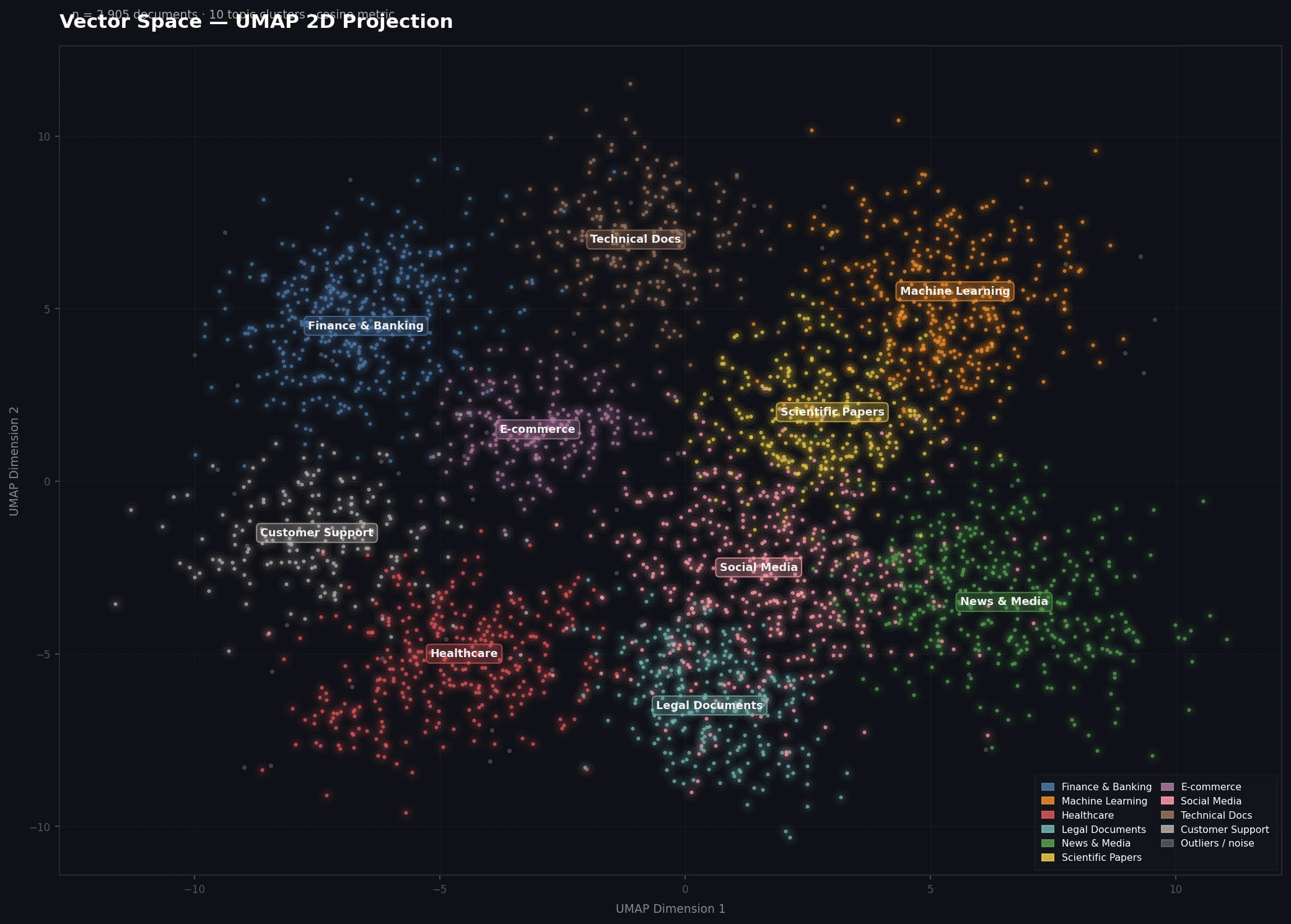UMAP projection showing distinct topic clusters Well-separated clusters indicate your embedding model is distinguishing topics correctly

Step 5: Speed Up Large Datasets

If you have 100k+ vectors, add these settings:

reducer = umap.UMAP(
    n_neighbors=15,
    min_dist=0.1,
    metric="cosine",
    low_memory=True,       # Reduces RAM at cost of speed
    n_jobs=-1,             # Use all CPU cores
    random_state=42
)

# For very large sets: approximate nearest neighbors
# Install: pip install pynndescent
# UMAP uses this automatically when installed

For production audits on millions of vectors, project a stratified sample of 50k first to get the lay of the land.

Verification

Run this end-to-end sanity check:

# Quick smoke test with random data
import numpy as np
import umap

dummy = np.random.randn(500, 128)  # 500 vectors, 128 dims
reducer = umap.UMAP(n_components=2, random_state=42)
out = reducer.fit_transform(dummy)
assert out.shape == (500, 2), "Shape mismatch"
print("UMAP working correctly.")

You should see: UMAP working correctly. in under 10 seconds.

What to Look For

Once you have the plot open, here's how to interpret what you see:

Tight, well-separated clusters — your embedding model is distinguishing categories cleanly. Retrieval should work well.

One giant blob — either your data is genuinely homogeneous, or your embedding model is too generic for this domain. Consider a domain-specific model.

Scattered outliers far from all clusters — probable mislabels, duplicates, or malformed documents. Worth inspecting those points by index:

# Find the most isolated points
from scipy.spatial.distance import cdist

center = projected.mean(axis=0)
distances = np.linalg.norm(projected - center, axis=1)
outlier_indices = np.argsort(distances)[-20:]  # Top 20 outliers
print(texts[outlier_indices])

Two similar clusters close together — your categories may overlap semantically. Consider merging them or using a finer-grained model.

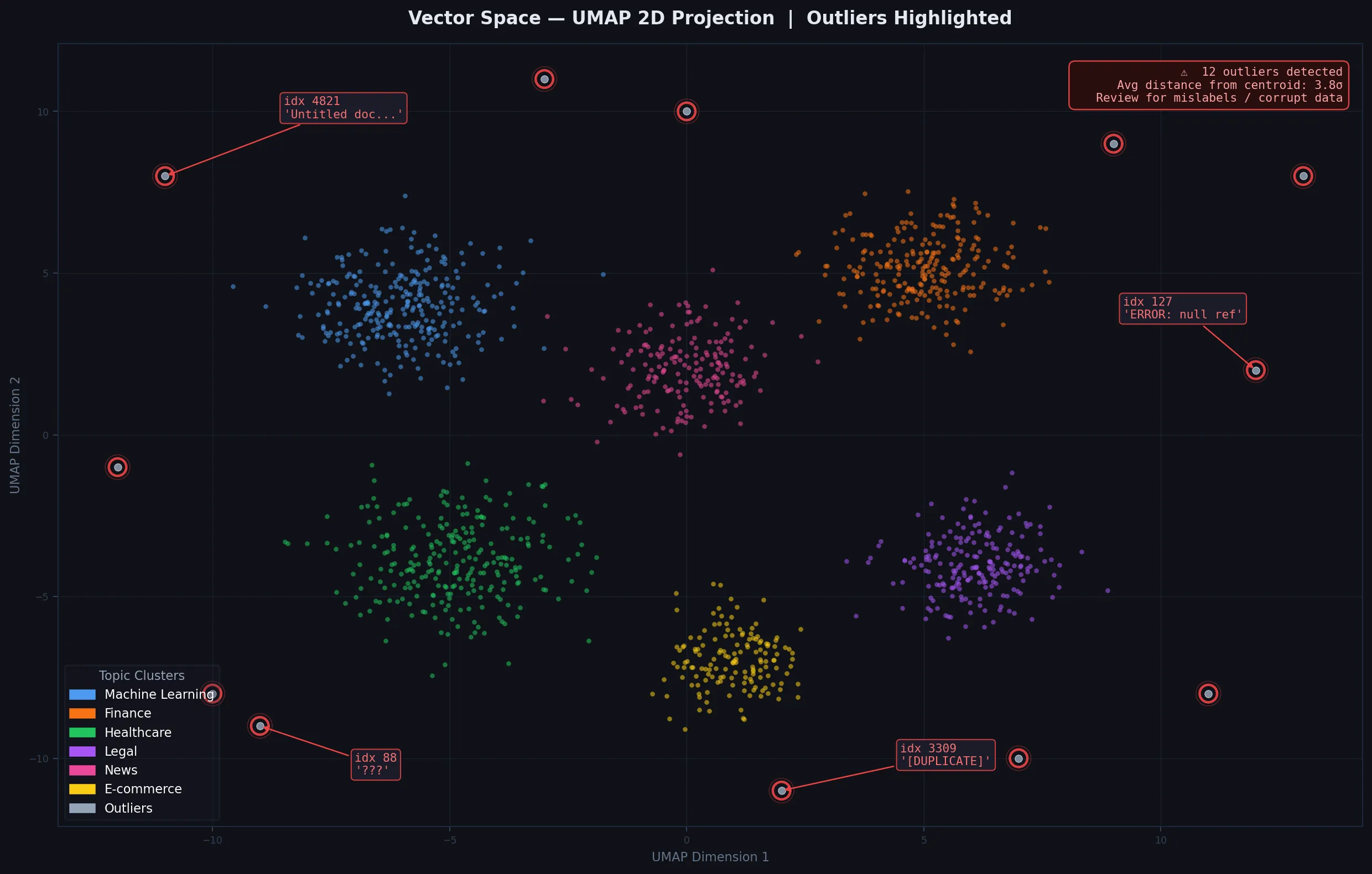UMAP showing outlier documents circled in red Isolated points far from clusters are worth reviewing for data quality issues

What You Learned

UMAP projects high-dimensional embeddings to 2D while preserving local cluster structure
metric="cosine" is the right choice for text embeddings
The interactive Plotly plot is significantly more useful than static matplotlib for exploration
Low min_dist shows tighter separation; high n_neighbors shows more global structure

Limitations to know:

UMAP layouts are non-deterministic unless you fix random_state — don't compare two plots without it
Distances in the 2D projection are not proportional to true cosine distances — only topology is preserved
On GPUs, use cuml.UMAP (RAPIDS) for 10-100x speedups on large datasets

When NOT to use this: If you need the actual low-dimensional vectors for downstream ML (not just visualization), PCA is faster and the output dimensions are interpretable.

Tested on Python 3.12, umap-learn 0.5.6, NumPy 1.26, Ubuntu 22.04 & macOS Sequoia