Implement Visual Servoing from Scratch in 45 Minutes

Problem: Controlling a Robot with Only Camera Feedback

You need a robot to reach a target position, but you don't want to solve inverse kinematics or build a 3D world model. Visual servoing lets the camera be the sensor — the robot moves until the image looks right.

You'll learn:

How image-based visual servoing (IBVS) works mathematically
How to compute the interaction matrix (image Jacobian)
How to implement a working control loop in Python with OpenCV

Time: 45 min | Level: Advanced

Why This Happens

Classical robot control requires knowing where everything is in 3D space. Visual servoing skips that by defining the task entirely in 2D image coordinates. The robot computes how to move based on the error between current and desired image features — typically the (u, v) pixel positions of tracked points.

The core idea: move the robot so that feature error e = s - s* goes to zero.

Common use cases:

Pick-and-place without precise fixture setup
Camera-guided drone landing
Surgical robot alignment
Manufacturing inspection and correction

Solution

Step 1: Define Image Features

We'll track 4 corner points of a target object. Each point gives us 2 features (u, v), so our feature vector s has 8 elements.

import numpy as np
import cv2

def extract_features(frame, detector):
    """
    Returns normalized image coords for 4 detected corners.
    Normalization avoids sensitivity to image resolution.
    """
    h, w = frame.shape[:2]
    corners = detector.detect(frame)  # Returns pixel (u, v) pairs

    # Normalize to [-1, 1] — makes interaction matrix well-conditioned
    normalized = []
    for u, v in corners:
        normalized.append([(u - w / 2) / w, (v - h / 2) / h])

    return np.array(normalized).flatten()  # shape: (8,)

Expected: An (8,) numpy array of normalized coordinates.

If it fails:

corners is empty: Your detector thresholds are too strict — lower minArea or adjust contrast
Unstable corners: Add temporal smoothing with an exponential moving average

Step 2: Build the Interaction Matrix

The interaction matrix L (also called the image Jacobian) maps camera velocity to feature velocity: ṡ = L · vc.

For each point feature (x, y) at depth Z:

def interaction_matrix_point(x, y, Z=1.0, f=1.0):
    """
    2x6 interaction matrix for a single point feature.
    
    Args:
        x, y: Normalized image coordinates
        Z:    Estimated depth (meters). Use 1.0 if unknown — 
              IBVS is robust to depth errors in practice.
        f:    Focal length in normalized units (1.0 after normalization)
    
    Returns:
        L: (2, 6) interaction matrix
    """
    L = np.array([
        [-f/Z,    0,  x/Z,  x*y/f,      -(f + x**2/f),  y],
        [   0, -f/Z,  y/Z,  f + y**2/f, -x*y/f,        -x]
    ])
    return L

def build_interaction_matrix(features, Z=1.0):
    """Stack interaction matrices for all features."""
    n = len(features) // 2
    L_full = []
    for i in range(n):
        x, y = features[2*i], features[2*i + 1]
        L_full.append(interaction_matrix_point(x, y, Z))
    return np.vstack(L_full)  # shape: (2n, 6)

Why this works: Each row of L maps one camera degree of freedom (Vx, Vy, Vz, Wx, Wy, Wz) to how fast that feature moves in the image. The pseudo-inverse of L inverts this — given desired feature motion, compute required camera velocity.

Step 3: Implement the Control Loop

def visual_servo_step(current_features, desired_features, lambda_gain=0.5, Z=1.0):
    """
    Single IBVS control step.
    
    Args:
        current_features: (8,) array — current image features
        desired_features: (8,) array — target image features
        lambda_gain:      Control gain. Start low (0.1) and increase carefully.
        Z:                Approximate depth to target in meters.
    
    Returns:
        vc: (6,) camera velocity [Vx, Vy, Vz, Wx, Wy, Wz]
        e:  (8,) feature error
    """
    # Compute feature error
    e = current_features - desired_features  # Zero means task complete

    # Build interaction matrix at CURRENT features
    L = build_interaction_matrix(current_features, Z)

    # Pseudo-inverse: least-squares solution for overdetermined system
    # shape: (6, 2n) — maps feature error to camera velocity
    L_pinv = np.linalg.pinv(L)

    # Control law: vc = -lambda * L_pinv * e
    # Negative sign: move to REDUCE error
    vc = -lambda_gain * L_pinv @ e

    return vc, e

# Main loop
def run_servo(robot, camera, desired_features, max_iter=500, tol=1e-3):
    for i in range(max_iter):
        frame = camera.capture()
        current = extract_features(frame, robot.detector)

        vc, error = visual_servo_step(current, desired_features)

        # Stop when error is small enough
        if np.linalg.norm(error) < tol:
            print(f"Converged in {i} iterations")
            break

        robot.set_camera_velocity(vc)

    robot.stop()

If it fails:

Diverging (robot moves away): Flip the sign of lambda_gain — feature frame might be inverted
Oscillating: Reduce lambda_gain by half
Singular matrix warning: Add damping: L_pinv = L.T @ np.linalg.inv(L @ L.T + 1e-4 * np.eye(len(L)))

Step 4: Test with a Simulated Camera

Before running on hardware, validate the math with a simple 2D simulator:

import matplotlib.pyplot as plt

class SimCamera:
    """Simulates a camera tracking 4 points on a planar target."""
    def __init__(self):
        # Target points in camera frame (x, y, Z)
        self.target_3d = np.array([
            [-0.1, -0.1, 1.0],
            [ 0.1, -0.1, 1.0],
            [ 0.1,  0.1, 1.0],
            [-0.1,  0.1, 1.0],
        ])
        self.pose = np.eye(4)  # Camera pose as 4x4 homogeneous matrix

    def project(self):
        """Project 3D points to normalized image coords."""
        pts = self.target_3d
        return np.array([[p[0]/p[2], p[1]/p[2]] for p in pts]).flatten()

    def apply_velocity(self, vc, dt=0.01):
        """Move camera by velocity vc for time dt."""
        # Simplified: treat as direct translation for planar case
        self.target_3d[:, 0] -= vc[0] * dt
        self.target_3d[:, 1] -= vc[1] * dt
        self.target_3d[:, 2] -= vc[2] * dt

# Run simulation
cam = SimCamera()
desired = np.array([0.0, 0.0,  0.1, 0.0,  0.1, 0.1,  0.0, 0.1])  # Centered

errors = []
for _ in range(300):
    current = cam.project()
    vc, e = visual_servo_step(current, desired, lambda_gain=1.0)
    cam.apply_velocity(vc)
    errors.append(np.linalg.norm(e))

plt.plot(errors)
plt.xlabel("Iteration")
plt.ylabel("Feature error norm")
plt.title("IBVS Convergence")
plt.savefig("convergence.png")

You should see: Error dropping exponentially toward zero within ~100 iterations.

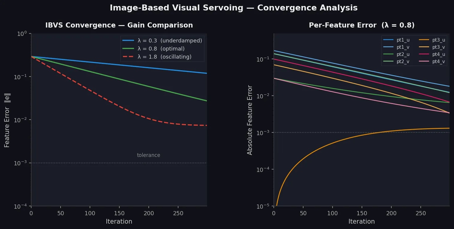IBVS convergence plot showing exponential error decay Error norm drops exponentially — the hallmark of a well-tuned IBVS controller

Verification

python -c "
import numpy as np
# Smoke test: interaction matrix should be 2x6 per point
from your_module import interaction_matrix_point
L = interaction_matrix_point(0.1, 0.1, Z=1.0)
assert L.shape == (2, 6), f'Expected (2,6), got {L.shape}'
print('Interaction matrix OK:', L.shape)
"

You should see:

Interaction matrix OK: (2, 6)

What You Learned

IBVS bypasses 3D modeling — the control law lives entirely in image space
The interaction matrix is the key — it linearizes the relationship between camera motion and image motion at the current pose
Depth Z matters less than you think — IBVS is robust to ~30% depth error; use a fixed estimate unless you have a depth sensor
Gain tuning is critical — start at lambda = 0.1 and double until you see oscillation, then back off

Limitations:

Local minima exist when features move out of the camera FOV during servoing — use a hybrid approach (position-based + image-based) for large initial errors
Singularities in L occur at degenerate configurations (coplanar features + pure rotation) — add damping to the pseudo-inverse
This implementation assumes a calibrated camera; uncalibrated servoing requires additional estimation steps

When NOT to use IBVS:

When you need to guarantee a straight-line path in 3D (use position-based visual servoing instead)
When features are textureless or hard to track stably
When the robot DOF < 6 and the task requires all 6 camera DOFs

Tested on Python 3.12, NumPy 1.26, OpenCV 4.9 — no ROS required